The Graphical Model Zoo
There are many ways to express complicated probability distributions. Some ways are more general than others.
This post collates the sources I used to make the figure depicting the hierarchy of probabilistic graphical models. Some excerpts have been pasted verbatim, but others are edited for readability. Please let me know if you find any errors in the hierarchy.
Energy-based models
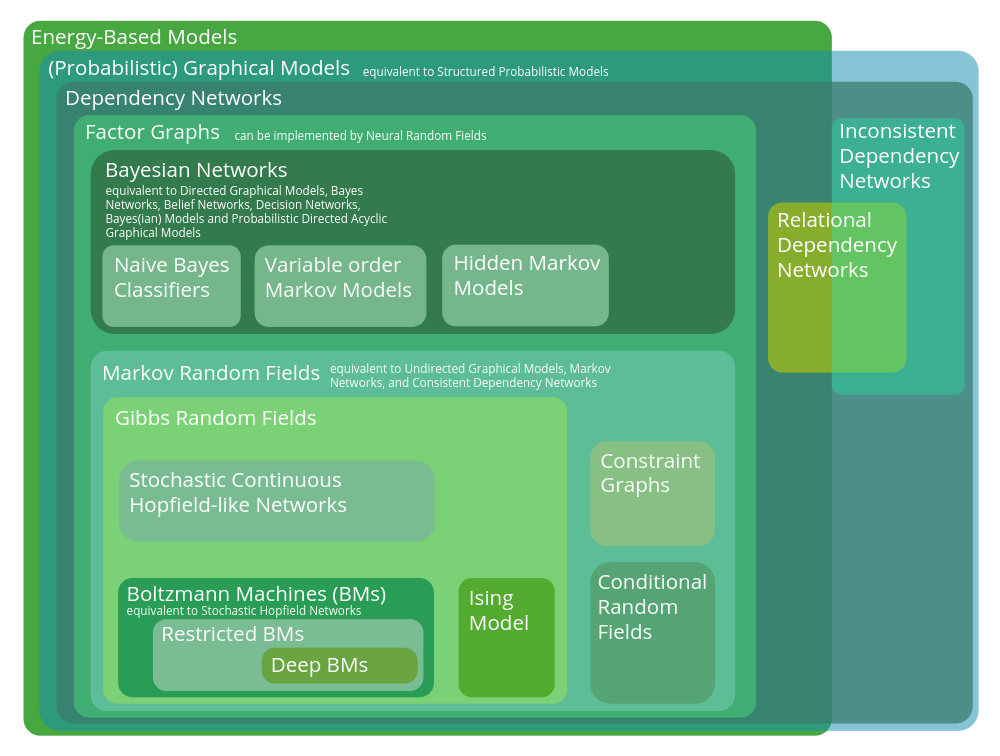
EBMs do not need to be expressed as a graph, but they often are, e.g. in Boltzmann Machines. Energy-Based Models (EBMs) describe dependencies between probabilistic variables by associating an energy (a scalar) to every possible configuration of the variables (LeCun et al., 2006). Any joint probability distribution can be defined in terms of a suitably expressive energy function, such as a graph that defines the conditional dependencies between variables. Hence, here we define EBMs as the largest class of models.
Sources:
- A Tutorial on Energy-Based Learning. LeCun et al. (2006).
[Probabilistic] Graphical Models
equivalent to Structured Probabilistic Models.
According to Bishop (Chapter 8), in a probabilistic graphical model, each node represents a random variable (or group of random variables), and the links express probabilistic relationships between these variables. The graph then captures the way in which the joint distribution over all of the random variables can be decomposed into a product of factors each depending only on a subset of the variables.
Sources:
- Pattern Recognition and Machine Learning. Bishop (2006)
Dependency Networks
The nodes in dependency networks consist of conditional probability tables, which determines the realization of the random variable given its parents.
Neville and Jensen (2007): “The primary distinction between Bayesian networks, Markov networks, and dependency networks (DNs) is that dependency networks are an approximate representation. DNs approximate the joint distribution with a set of conditional probability distributions (CPDs) that are learned independently. This approach to learning results in significant efficiency gains over exact models. However, because the CPDs are learned independently, DNs are not guaranteed to specify a consistent joint distribution, where each CPD can be derived from the joint distribution using the rules of probability.”
Sources:
- Wikipedia, Dependency Networks
- Dependency Networks for Inference, Collaborative Filtering, and Data Visualization. Heckerman et al. Journal of Machine Learning Research 1 (2000) 49-75.
- Relational Dependency Networks. Neville and Jensen. Journal of Machine Learning Research 8 (2007) 653-692
Relational Dependency Networks
Wikipedia: Relational dependency networks (RDNs) are graphical models which extend dependency networks to account for relational data. Relational data is data organized into one or more tables, which are cross-related through common fields. A relational database is the canonical example of a system that serves to maintain relational data. A relational dependency network can be used to characterize the knowledge contained in a database.
Sources:
- Wikipedia, Relational dependency network
- Relational Dependency Networks. Neville and Jensen. Journal of Machine Learning Research 8 (2007) 653-692
Factor Graphs
The Hammersley–Clifford theorem shows that Bayesian networks and Markov Random Fields can be represented as factor graphs.
Sources:
- Wikipedia, Factor Graph
- An Introduction to Factor Graphs. Hans-Andrea Loeliger. IEEE Signal Processing Mag., Jan. 2004
- Factor Graphs and the Sum-Product Algorithm. F. R. Kschischang, B. J. Frey and H-A. Loeliger. IEEE Transactions on Information Theory, vol. 47, no. 2, pp. 498-519, Feb 2001.
Markov Random Fields
equivalent to Undirected Graphical Models, Markov Networks, and Consistent Dependency Networks
The Hammersley–Clifford theorem implies that Markov Random Fields can be expressed as factor graphs. Loeliger (2004) demonstrates equivalent ways to express MRFs as factor graphs. Heckerman et al. (2000) show how they are equivalent to consistent dependency networks.
Sources:
- Wikipedia, Markov Random Fields.
- Dependency Networks for Inference, Collaborative Filtering, and Data Visualization. Heckerman et al. Journal of Machine Learning Research 1 (2000) 49-75.
- An Introduction to Factor Graphs. Hans-Andrea Loeliger. IEEE Signal Processing Mag., Jan. 2004
Bayesian Networks
equivalent to Directed Graphical Models, Bayes Networks, Belief Networks, Decision Networks, Bayes(ian) Models and Probabilistic Directed Acyclic Graphical Models.
The Hammersley–Clifford theorem implies that Bayesian networks can be expressed as factor graphs. Loeliger (2004) demonstrates equivalent ways to express Bayesian nets as factor graphs.
Sources:
- Wikipedia, Bayesian Network.
- Wikipedia, Factor Graph
- An Introduction to Factor Graphs. Hans-Andrea Loeliger. IEEE Signal Processing Mag., Jan. 2004
Hidden Markov Model & Naive Bayes Classifiers & Variable-order Markov models
Each is a special case of Bayesian networks. Sources:
Gibbs Random Field
In a Markov Random Field where the joint probability density of the random variables is positive everywhere, it is also referred to as a Gibbs random field, because, according to the Hammersley–Clifford theorem, it can then be represented by a Gibbs measure for an appropriate (locally defined) energy function.
Sources:
Constraint Graph
Factor graphs are generalisations of constraint graphs. As far as I can see, no other class of graphical model can be expressed in terms of a constraint graph, but I could easily be wrong; I couldn’t find any good, free sources on constraint graphs.
Sources:
Conditional Random Field
A variant of a Markov Random Field where each random variable can be conditioned on a set of global observations.
Sources:
- Wikipedia, Conditional Random Field.
- Conditional Random Fields: Probabilistic models for segmenting and labeling sequence data. Lafferty, McCallum, and Pereira (2001). Proc. 18th International Conf. on Machine Learning. Morgan Kaufmann. pp. 282–289.
Ising Model
The Ising model is the canonical Markov random field; indeed, the Markov random field was introduced as the general setting for the Ising model by Kindermann and Snell (1980).
Sources:
- Wikipedia, Markov Random Fields.
- Wikipedia, Ising Model.
- Markov Random Fields and their applications. Kindermann and Snell (1980). American Mathematical Society. ISBN 978-0-8218-5001-5. MR 0620955.
Neural Random Field
Neural random fields are defined by using neural networks to implement potential functions in Markov random fields. Sources:
- Learning Neural Random Fields with Inclusive Auxiliary Generators. Song and Ou 2018. arXiv:1806.00271
Continuous Hopfield-like Networks
These include networks such as the EBM first studied by Bengio and Fischer (2015), where the neural network used to implement the conditional dependencies between variables is a linear network. The overall network is nevertheless nonlinear due to the saturating threshold functions that constrain the variables to [0,1].
Sources:
- Early Inference in Energy-Based Models Approximates Back-Propagation. Bengio and Fischer. arXiv e-prints, abs/1510.02777
Boltzmann Machine
A Boltzmann machine of finite size is a Gibbs random field if weights of infinite magnitude are disallowed, since the energy can thus not be infinite and therefore the joint probability density is positive everywhere.
They are the stochastic version of the original Hopfield Networks.
Sources: